
Converts the image to greyscale, this calculates the luminosity of each
pixel by averaging red, green and blue values.
Since currently many filters work on grayscale images only, this is
useful.
The "small" convolution engine is now ready and functional.
By entering a 5x5 matrix you can specify a FIR (Finite Impulse
Response) filter that will be applied on the image. Since usually the
dynamic range will exceed the available 8 bit range, you can either
specify an offest and a scale (the over or undershooting will be
clipped) or activate the autoscale algorithm.
Intuitively the filter works by sweeping over the image, summing up all
samples of the image under the filter area after having multiplied them
by the entity of the pixel sample and putting back the result in the
sample under the centre of the pixel.To avoid phase shifts in the
filter (which means that the imga moves after the application of the
filter) it is adivsable to keep the filter symmetric against the middle
sample. To preserve the energy (brightness) of the image, the sum of
all samples of the filter should be 1; if it is 0 only the features
extracted by the filter are visible (useful for example to extract
edges). Since usually filters modify the brightness you can choose to
either try to adjust the range manually (using the scale and offest
paramteres) or attempt an autoscale to display the full dynamic range
compressed: although the latter may be mathematically more correct
since no clipping occours, it can have undesired effects, especially
with high-pass filters.
For example you can trace some edges using a filter that approximates the laplacian (about the second derivative of an image).
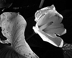
This is the original image:

A first version uses the four neighbors of a pixel
| 0 | -1 | 0 |
| -1 | 4 | -1 |
| 0 | -1 | 0 |
This will calculate where the image's grey gradinets change sign. SInce we are calculating a derivative function, we expect to have the constant parts disappear and the output will have a positive and negative output. We can either scale and shift the result, so to have the 0 shifted to a grey or we can clip what exceeds the [0, 1) interval.
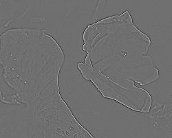
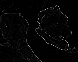
Adding 1 at the center preserves the image itself and superimposes the effect of the filter (roughly said) and voilà... you have some sort of image enhancing. Using The following matrix we obtain the typical sharpen edges effect.
|
 |
Calculates and displays the DFT (Discrete Fourier Transform) using the FFT algorithm. Only Greyscale images are accepted and the result is displayed shifted so that the origin is in the center. The output is a logarithmic representation of the square modulus of the transform.
The DFT represents an image in its frequency components. I will explain
some simple properties in the 1D case.
The DFT essentially calculates how a sequence (representing the
discrete form of a signal) resembles to the forms of a choosen basic
function, in this case a series of sines and cosines at different
frequencies. So every coefficient is related to sinusoidal funciton at
a certain frequency and its value represents "how much of that
sinusoid is present in the signal".
So a signal composed of a single sinus at a certain frequency will have
a foruier transform that is all zero except for one point: the one
representing that exact frequency. A signal composed of the sum of thwo
sinusoids will have 2 non zero values. The fourier transform operates
on continuous and periodic signals. When operating discrete and finite
sequences we can think that the piece of sequence we have represents
one single period of a periodic function. In the case of the 2D the DFT
operates first horizontally and then vertically (this means the
calculation of the DFT is separable) and so this periodicization can be
thought as considering the image as one tile of a floor of repetitions.
Some consideration about basic transforms:
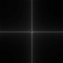
Bearing in mind these simple properties one can better understand some simple examples. Also useful to remember that since the FFT is calculated by rows and colums, if an image is constant in one direction (a so-called cylindrical function), the transform will be non-zero only in the origin in one direction and will represent the 1D transform of the function in the other (like a slice).
Please note that the full tranform of an image is a complex result . This means that it needs to be represented by a Real and Imaginary part, both ranging from -inf to +inf! The result that PRICE displays is the logarithm of the square modulus rised by one. [f = log(sqr(x) + 1] Also PRICE performs an FFT-shift to display the origin of the axes in the centre and not top-left ast the DFT would provide.
For the abovementioned reasons, PRICE cannot calculate the inverse FFT from the FFT result that it displays. Of course, when PRICE uses the FFT internally to calculate filters it keeps track of all necessary information to retransform back the original image without loss.
 |
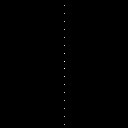 |
horizontal stripes show how the sequence is constant in one direction |
 |
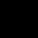 |
the other way |
 |
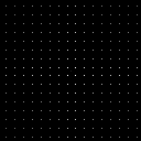 |
a checker is regular in both directions |
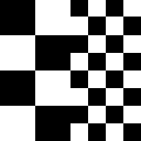 |
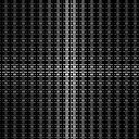 |
checkers with different frequencies |
 |
 |
|
 |
 |
a shifted impulse shows only the modulating part |
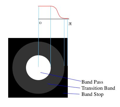
This filter selects the low frequencies of an image, creating what is
commonly called a "blur". The user an select, for the low
pass for example, the frequency up ot which the filter is passband and
where the stop-band begins. The Intermediate band between the two
regions is used as transition, to improve the smoothness of the filter,
currenlty the front of the filter is smoothed by a cosine in the
transition band. The filter is then calculated with circular symmetry.
A low pass filter gives the impression of blurring the image, while a
high pass extracts the details of an image, enhancing the transition
but turning uniform areas to grey.
 |
Original Image |
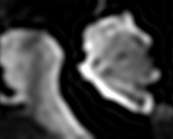 |
BandPass = 0.1*pi |
 |
BandPass = 0.1*pi |
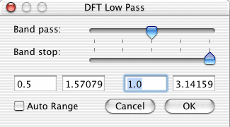 |
The dialog box: The boxes at left represent the band pass frequency, the ones at right the band stop. Values can be entered from the text widgets or by interactively moving the sliders.The two widgets for each frequency represent the value without and with pi. |
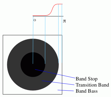
This filter selects the high frequencies of an image, commonly perceived as details and edges. As in the Low Pass filter, the band stop and band frequencies can be selected and the intermediate region is given by the gab of those two frequencies. Since a high-pass filter tends to remove the low frequencies, including f=0, the DC value (that is, the average value of the image which represents its brightness) the image tends to loose the average value and display higher contrast on the details. Since the detail would show up as ether positive or negative, they are either clipped or auto-ranged, that is the average value drifts to grey to be able to display all the details.
 |
Original Image |
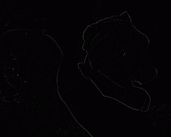 |
Band Stop = 0 An extremely smooth filter, which stops only DC and uses the whole (o, pi) range for transition. No auto-range |
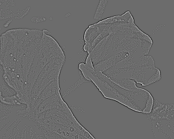 |
The same filter as above, but with auto-range enabled. |
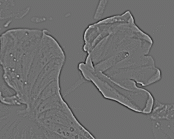 |
Band Stop = 0 |
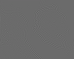 |
Band Stop = 0.25 |